Basic Ncut

TL;DR

1. Feature Extraction: Extract feature from pre-trained model (DINO, SAM, etc).
2. Affinity Graph: Compute feature similarity between nodes (pixels), build graph.
3. Ncut: Compute Ncut eigenvectors of the graph Laplacian.

---

Normalized Cuts and Spectral Clustering

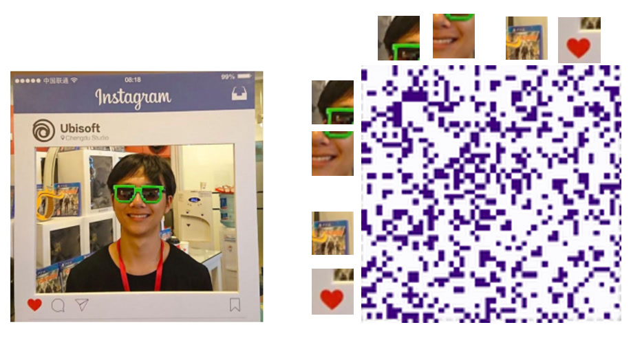
Spectral clustering, or Normalized Cuts, clusters data based on the eigenvectors (spectrum) of a similarity matrix derived from the data. The Normalized Cuts algorithm aims to partition a graph into subgraphs while minimizing the graph cut value.

Image taken from Spectral Clustering: Step-by-step derivation of the spectral clustering algorithm including an implementation in Python

---

The Basic Idea

Spectral clustering works by embedding the data points \(F \in \mathbb{R}^{N \times 768}\) into a lower-dimensional space using the eigenvectors of a Laplacian matrix derived from the data's similarity graph \(W \in \mathbb{R}^{N \times N}\). The data is then clustered in this new space embedded by \(k\) eigenvectors \(\mathbf{x} \in \mathbb{R}^{N \times k}\).

The Graph Laplacian

Given a set of data points, spectral clustering first constructs a similarity graph. Each node represents a data point, and edges represent the similarity between data points. The similarity graph can be represented by an adjacency matrix \( W \), where each element \( W_{ij} \) represents the similarity between data points \( i \) and \( j \).

Take cosine distance for example, let \(F \in \mathbb{R}^{N \times 768}\) be the input features (from a backbone image model), \(N\) is number of pixels, \(768\) is feature dimension. Feature vectors \(f_i, f_j \in \mathbb{R}^{768}\), the cosine similarity between \(f_i\) and \(f_j\) is defined as:

\[W_{ij} = \text{cosine}(f_i, f_j) = \frac{f_i \cdot f_j}{|f_i| |f_j|}\]

where \(|f|\) denotes the Euclidean norm of a vector \(f\).

In matrix form, this can be written as:

\[W = \text{cosine}(F, F) = \frac{F F^\top}{\text{diag}(F F^\top)^{1/2} , \text{diag}(F F^\top)^{1/2}}\]

where \(F F^\top \in \mathbb{R}^{N \times N}\) is the matrix of pairwise dot products between the feature vectors, and \(\text{diag}(\cdot)\) extracts the diagonal elements of a square matrix. The resulting matrix \(W = \text{cosine}(F, F)\) is an \(\mathbb{R}^{N \times N}\) matrix, where each element \((i, j)\) represents the cosine similarity between the \(i\)-th and \(j\)-th feature vectors.

The degree matrix \( D \) is a diagonal matrix where each element \( D_{ii} \) is the sum of the similarities of node \( i \) to all other nodes.

\[ D_{ii} = \sum_{j=0}^{N} W_{ij} \]

The unnormalized graph Laplacian is:

\[ L = D - W \]

The normalized graph Laplacian has two common forms:

1. Symmetric normalized Laplacian:

\[ L_{\text{sym}} = D^{-1/2} L D^{-1/2} = I - D^{-1/2} W D^{-1/2} \]

1. Random walk normalized Laplacian:

\[ L_{\text{rw}} = D^{-1} L = I - D^{-1} W \]

Normalized Cuts

Normalized Cuts (Ncut) is a method for partitioning a graph into disjoint subsets, aiming to minimize the total edge weight between the subsets relative to the total edge weight within each subset. The Ncut criterion is particularly useful for ensuring balanced partitioning, which prevents trivial solutions where one cluster might be significantly smaller than the other.

The normalized cut criterion is defined as:

\[ \text{Ncut}(A, B) = \left(\frac{\text{cut}(A, B)}{\text{assoc}(A, V)}\right) + \left(\frac{\text{cut}(A, B)}{\text{assoc}(B, V)}\right) \]

Where:

• \( A \) and \( B \) are two disjoint subsets (clusters) of the graph.

• \( \text{cut}(A, B) \) is the sum of the weights of the edges between the subsets \( A \) and \( B \):

\[ \text{cut}(A, B) = \sum_{i \in A, j \in B} W_{ij} \]

• \( \text{assoc}(A, V) \) is the sum of the weights of all edges attached to nodes in subset \( A \) (similar definition for \( B \)):

\[ \text{assoc}(A, V) = \sum_{i \in A, j \in V} W_{ij} \]

The goal is to find a partition that minimizes the Ncut value, which balances minimizing the inter-cluster connection (cut) with maintaining strong intra-cluster connections (association).

Solving the Normalized Cut Using Eigenvectors

To solve the Ncut problem, we reformulate it as a problem of finding the eigenvectors of a normalized graph Laplacian. Here’s how this works:

Mathematical Formulation

Let \( \mathbf{x} \) be an indicator vector such that:

\[ x_i = \begin{cases} 1 & \text{if node } i \in A \\ -1 & \text{if node } i \in B \end{cases} \]

The cut value \( \text{cut}(A, B) \) can be rewritten in terms of \( \mathbf{x} \) as:

\[ \text{cut}(A, B) = \frac{1}{4} \sum_{i,j} W_{ij} (x_i - x_j)^2 = \mathbf{x}^\top L \mathbf{x} \]

Where \( L = D - W \) is the unnormalized graph Laplacian.

The association \( \text{assoc}(A, V) \) is given by:

\[ \text{assoc}(A, V) = \mathbf{x}^\top D \mathbf{1}_A \]

Here, \( \mathbf{1}_A \) is a vector that is 1 for elements in \( A \) and 0 elsewhere.

The Ncut problem can thus be rewritten as:

\[ \text{Ncut}(A, B) = \frac{\mathbf{x}^\top L \mathbf{x}}{\mathbf{x}^\top D \mathbf{x}} \]

Minimizing this directly is NP-hard. However, it can be relaxed into a generalized eigenvalue problem, because the above eq is close to the Rayleigh quotient which is minimized by solving eigenvectors. By relaxing the constraint that \( x_i \) takes only discrete values (1 or -1), we allow \( \mathbf{x} \) to take real values, and the problem becomes finding the eigenvector corresponding to the second smallest eigenvalue of the generalized eigenvalue problem:

\[ L \mathbf{y} = \lambda D \mathbf{y} \]

To make it a simple eigenvalue solving, that can be solved by most eigenvector solvers. Move \(D\) to the left side of the equation. this is equivalent to finding the eigenvectors of the normalized Laplacian:

\[ D^{-1/2} L D^{-1/2} \mathbf{y} = \lambda \mathbf{y} \]

Proof of Minimization

The eigenvector approach is derived from the relaxation of the original NP-hard problem. By solving the generalized eigenvalue problem:

\[ L \mathbf{y} = \lambda D \mathbf{y} \]

We are effectively minimizing the Rayleigh quotient:

\[ \frac{\mathbf{y}^\top L \mathbf{y}}{\mathbf{y}^\top D \mathbf{y}} = \frac{\mathbf{y}^\top D^{-1/2} L D^{-1/2} \mathbf{y}}{\mathbf{y}^\top \mathbf{y}} \]

The Rayleigh quotient directly reflecting the Ncut objective. The solution of Rayleigh quotient is eigenvectors

\[ \text{Ncut}(A, B) = \frac{\mathbf{x}^\top L \mathbf{x}}{\mathbf{x}^\top D \mathbf{x}} = \frac{\mathbf{x}^\top D^{-1/2} L D^{-1/2} \mathbf{x}}{\mathbf{x}^\top \mathbf{x}} \]

thus, solving eigenvector \(\mathbf{y}\) of \(D^{-1/2} L D^{-1/2} = \lambda \mathbf{y}\) is equal to solving the graph cut solution \(\mathbf{x}\):

\[ \mathbf{x} = \mathbf{y} \]

Laplacian vs Affinity

Normalized Cuts can also be solved by eigenvectors of \(D^{-1/2} W D^{-1/2} \), instead of \(D^{-1/2} L D^{-1/2} \), where \(L = D - W\). They have the same eigenvectors:

\[\begin{aligned} D^{-1/2} (D - W) D^{-1/2} &= Y \Lambda Y^T \\ I - D^{-1/2} W D^{-1/2} &= Y \Lambda Y^T \\ D^{-1/2} W D^{-1/2} &= Y (I - \Lambda) Y^T \end{aligned}\]

Eigenvectors and Clustering

The eigenvector corresponding to the second smallest eigenvalue (also called the Fiedler vector) provides a real-valued solution to the relaxed Ncut problem. Sorting the nodes based on the values in this eigenvector and choosing a threshold to split them yields an approximate solution to the Ncut problem.

Each subsequent eigenvector can be used to further partition the graph into subclusters. The process is as follows:

1. Compute the symmetric normalized Laplacian \( L_{\text{sym}} \).
2. Compute the eigenvectors \( \mathbf{x}_1, \mathbf{x}_2, \dots, \mathbf{x}_k \) corresponding to the smallest \( k \) eigenvalues.
3. Use \( \mathbf{x}_2 \) (the Fiedler vector) to divide the graph into two clusters.
4. For multi-way clustering, use the next eigenvectors \( \mathbf{x}_3, \mathbf{x}_4, \dots \) to further hierarchically subdivide these clusters.

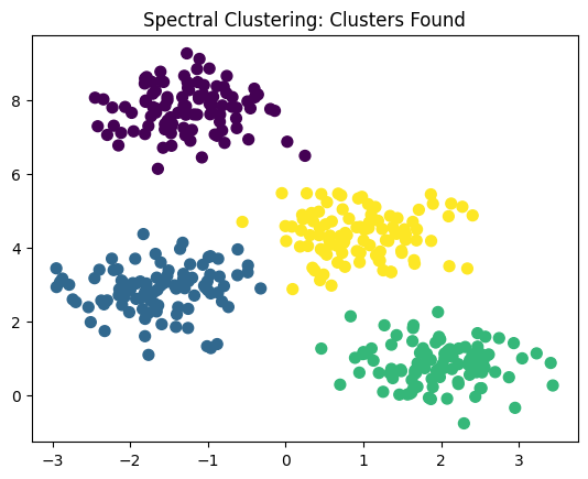
Example: Eigenvector Visualization

Let's visualize how the eigenvectors divide the graph into clusters using our toy example.

import numpy as np
import matplotlib.pyplot as plt
from sklearn.datasets import make_blobs
from scipy.linalg import eigh
from sklearn.metrics.pairwise import rbf_kernel
from sklearn.cluster import KMeans

# Generate synthetic data with 4 clusters
X, y = make_blobs(n_samples=400, centers=4, cluster_std=0.60, random_state=0)

# Compute the similarity matrix using RBF (Gaussian) kernel
sigma = 1.0
W = rbf_kernel(X, gamma=1/(2*sigma**2))

# Degree matrix
D = np.diag(np.sum(W, axis=1))

# Unnormalized Laplacian
L = D - W

# Normalized Laplacian (symmetric)
D_inv_sqrt = np.linalg.inv(np.sqrt(D))
L_sym = np.dot(np.dot(D_inv_sqrt, L), D_inv_sqrt)

# Compute the eigenvalues and eigenvectors of the normalized Laplacian
eigvals, eigvecs = eigh(L_sym)

# Plot the first few eigenvectors
k = 4  # number of clusters
for i in range(1, k+1):
    plt.figure()
    plt.scatter(X[:, 0], X[:, 1], c=eigvecs[:, i-1], s=50, cmap='coolwarm')
    plt.title(f"Eigenvector {i} - Dividing the Graph")
    plt.colorbar()
    plt.show()

# Use the first k eigenvectors to form a matrix U
U = eigvecs[:, :k]

# Normalize U
U_norm = U / np.linalg.norm(U, axis=1, keepdims=True)

# Perform k-means clustering on U_norm
kmeans = KMeans(n_clusters=k, random_state=0)
labels = kmeans.fit_predict(U_norm)

# Plot the clusters
plt.scatter(X[:, 0], X[:, 1], c=labels, s=50, cmap='viridis')
plt.title("Spectral Clustering: Clusters Found")
plt.show()

• The 1-st eigenvector generally corresponds to the global structure (often related to the connected components of the graph).

• The 2-nd eigenvector splits the graph into 2 clusters.

• Subsequent eigenvectors further hierarchically splits the data into more detailed sub-clusters.

A Good Eigenvector Solver

Solving the full eigenvector \(\mathbf{x} \in \mathbb{R}^{N \times N}\) is computational expensive, methods has been developed to solve top k eigenvectors \(\mathbf{x} \in \mathbb{R}^{N \times k}\) in linearly complexity scaling. In particular, we use svd_lowrank.

• Reference:

  Nathan Halko, Per-Gunnar Martinsson, and Joel Tropp, Finding structure with randomness: probabilistic algorithms for constructing approximate matrix decompositions, 2009.

Summary

The Normalized Cuts algorithm aims to partition a graph into subgraphs while minimizing the graph cut value. It embeds the data points into a lower-dimensional space using the eigenvectors of a Laplacian matrix derived from the data's similarity graph.

---

Previous ← Methods Overview Back to Overview Next Nyström NCut (Complexity) →