Nyström Ncut (Complexity)
TL;DR
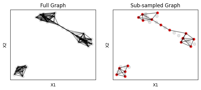
- Sub-sample: Solve Ncut on a smaller sub-sampled graph, reduce complexity.
- kNN Propagation: Propagate the Ncut values from sampled nodes to not-sampled.
The Nyström Ncut approximation dramatically improves computational complexity from quadratic to linear time complexity O(N), making it feasible to process large-scale graphs with millions of nodes.
How Nyström Ncut works
An intuition: Nystrom approximation solve the large-scale problem on a small sub-sampled set, then propagate the solution from the small set to the large set.
The approach involves three main steps: (1) sub-sampling a subset of nodes, (2) computing the Normalized Cut (Ncut) on the sampled nodes, and (3) propagating the eigenvectors from the sampled nodes to the unsampled nodes.
Sub-sampling the Affinity Matrix
The affinity matrix \( W \) is partitioned as follows:
where:
-
\( A \in \mathbb{R}^{n \times n} \) is the submatrix of weights among the sampled nodes,
-
\( B \in \mathbb{R}^{(N-n) \times n} \) is the weights between the sampled nodes and the remaining unsampled nodes,
-
\( C \in \mathbb{R}^{(N-n) \times (N-n)} \) is the weights between the unsampled nodes.
Computation loads: \( C \) is a very large matrix that is computationally expensive to handle. \( B \) is also expensive to store and compute once sampled nodes \( n \) gets large, although \( n \) (the number of sampled nodes) is much smaller than \( N \) (the total number of nodes), a better quality of Nystrom approximation requires \( n \) to be larger, thus makes \( B \) a large matrix.
k-Nearest Neighbors (kNN) Propagation
Farthest Point Sampling (FPS) is used to select nodes that are evenly distributed across the data, we use fpsample.
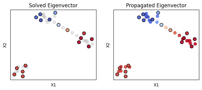
After computing the eigenvectors \( \mathbf{X}' \in \mathbb{R}^{n \times C} \) on the sub-sampled graph \( S = A + \left({D_{\text{r}}}^{-1} B'\right) \left(B' {D_{\text{c}}}^{-1}\right)^\top \in \mathbb{R}^{n \times n} \) using the Ncut formulation, the next step is to propagate these eigenvectors to the full graph. Let \( \mathbf{\tilde{X}} \in \mathbb{R}^{N \times C} \) be the approximated eigenvectors for the full graph, where \( N \) is the total number of nodes. The eigenvector approximation \( \mathbf{\tilde{X}}_i \) for each node \( i \leq N \) in the full graph is obtained by averaging the eigenvectors \( \mathbf{X}'_k \) of the top K-nearest neighbors from the subgraph:
Here, \( \text{KNN}(\mathbf{A}_{*i}; n, K) \) denotes the set of K-nearest neighbors from the full-graph node \( i \leq N \) to the sub-graph nodes \( k \leq n \). In other words, the eigenvectors of un-sampled nodes are assigned by weighted averaging top KNN eigenvectors from sampled nodes.