Inference and Extrapolation
Once an NCUT model is fitted, it is possible to extrapolate the spectral embedding to new data points. New nodes are assigned eigenvectors and colors via Nyström propagation. This means the new nodes are treated as if they were not sampled during the approximation but are added to the graph through propagation. This approach is effective when the original sampled nodes provide good coverage of the newly added nodes.
Feature Extraction
First, we extract features for a base set of images.
Click to expand full code
import torchvision
import torch
from torchvision import transforms
from PIL import Image
import numpy as np
from einops import rearrange
from torch import nn

# Load Dataset
dataset_voc = torchvision.datasets.VOCSegmentation(
    "/data/pascal_voc/",
    year="2012",
    download=True,
    image_set="val",
)
print("Number of images in the dataset:", len(dataset_voc))

def feature_extractor(images, resolution=(448, 448), layer=11):
    if isinstance(images, list):
        assert isinstance(images[0], Image.Image), "Input must be a list of PIL images."
    else:
        assert isinstance(images, Image.Image), "Input must be a PIL image."
        images = [images]

    transform = transforms.Compose(
        [
            transforms.Resize(resolution),
            transforms.ToTensor(),
            transforms.Normalize([0.485, 0.456, 0.406], [0.229, 0.224, 0.225]),
        ]
    )

    # Extract DINOv2 last layer features
    class DiNOv2Feature(torch.nn.Module):
        def __init__(self, ver="dinov2_vitb14_reg", layer=11):
            super().__init__()
            self.dinov2 = torch.hub.load("facebookresearch/dinov2", ver)
            self.dinov2.requires_grad_(False)
            self.dinov2.eval()
            self.dinov2 = self.dinov2.cuda()
            self.layer = layer

        def forward(self, x):
            out = self.dinov2.get_intermediate_layers(x, reshape=True, n=np.arange(12))[
                self.layer
            ]
            return out

    feat_extractor = DiNOv2Feature(layer=layer)

    feats = []
    for i, image in enumerate(images):
        torch_image = transform(image)
        feat = feat_extractor(torch_image.unsqueeze(0).cuda()).cpu()
        feat = feat.squeeze(0).permute(1, 2, 0)
        feats.append(feat)
    feats = torch.stack(feats).squeeze(0)
    return feats
# Create a large-scale feature matrix
images = [dataset_voc[i][0] for i in range(100)]
feats = feature_extractor(images, resolution=(336, 336), layer=9)
print("Feature shape for 100 images:", feats.shape)
num_nodes = np.prod(feats.shape[:3])
print("Number of nodes for 100 images:", num_nodes)

# Sample Output:
# Feature shape for 100 images: torch.Size([100, 32, 32, 768])
# Number of nodes for 100 images: 102400
NCUT on Original Images
We fit the Ncut model on the original images. We keep the ncut_model instance to transform new data later.
from ncut_pytorch import Ncut

input_feats = feats.flatten(0, 2)

# Initialize and fit Ncut
ncut_model = Ncut(n_eig=20)
eigenvectors = ncut_model.fit_transform(input_feats)
Click to expand visualization code
import matplotlib.pyplot as plt
from PIL import Image

def plot_images(images, rgb, title):
    fig, axs = plt.subplots(4, 8, figsize=(10, 4))
    for i_row in range(0, 4, 2):
        for i_col in range(8):
            ax = axs[i_row, i_col]
            image = images[i_row * 4 + i_col]
            image = image.resize((224, 224), Image.BILINEAR)
            ax.imshow(image)
            ax.axis("off")
        for i_col in range(8):
            ax = axs[i_row + 1, i_col]
            ax.imshow(rgb[i_row * 4 + i_col])
            ax.axis("off")
    plt.suptitle(title, fontsize=16)
    plt.show()
# Apply t-SNE for visualization of the eigenvectors
from ncut_pytorch.color import tsne_color

rgb = tsne_color(
    eigenvectors[:, :20], perplexity=100, device="cuda:0",
)

image_rgb = rgb.reshape(feats.shape[:3] + (3,))
plot_images(images, image_rgb, "NCUT, Original Images")

Feature Extraction for New Images
We extract features for a new set of images (e.g., from index 1000 to 1100).
new_images = [dataset_voc[i][0] for i in range(1000, 1100)]
new_feats = feature_extractor(new_images, resolution=(336, 336), layer=9)
print("Feature shape for new images:", new_feats.shape)
Propagate Eigenvectors to New Images
Using the fitted ncut_model, we transform the new features to obtain their eigenvectors. We then propagate the colors from the original eigenvectors to the new ones to maintain consistent coloring.
from ncut_pytorch.ncuts import nystrom_propagate

# 1. Propagate eigenvectors to new data using the Ncut model
new_eigenvectors = ncut_model.transform(new_feats.reshape(-1, new_feats.shape[-1]))

# 2. Propagate RGB colors to new data based on eigenvector similarity
# We use nystrom_propagate to find neighbors in eigenvector space and average their colors
# nystrom_out: source values (rgb)
# X: target features (new_eigenvectors)
# nystrom_X: source features (eigenvectors)
new_rgb = nystrom_propagate(
    nystrom_out=rgb,
    X=new_eigenvectors[:, :20],
    nystrom_X=eigenvectors[:, :20],
    n_neighbors=10,
    device="cuda:0"
)

plot_images(
    new_images,
    new_rgb.reshape(new_feats.shape[:3] + (3,)).cpu(),
    "NCUT, Added Images (Propagated)",
)

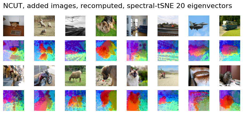
Comparison: Recompute vs. Propagate
Recomputing eigenvectors on the new data alone may result in better segmentation quality for those specific images, but the coloring (spectral embedding space) will not be consistent with the previous images, making comparison difficult.
# Recompute NCUT from scratch for new images
recomputed_eigenvectors = Ncut(n_eig=50).fit_transform(new_feats.reshape(-1, new_feats.shape[-1]))

# Recompute t-SNE colors
recomputed_rgb = tsne_color(
    recomputed_eigenvectors[:, :20], perplexity=100, device="cuda:0",
)

plot_images(
    new_images,
    recomputed_rgb.reshape(new_feats.shape[:3] + (3,)),
    "NCUT, Added Images (Recomputed)",
)